Raspberry Pi GoPiGo Robot EKF SLAM

Abstract

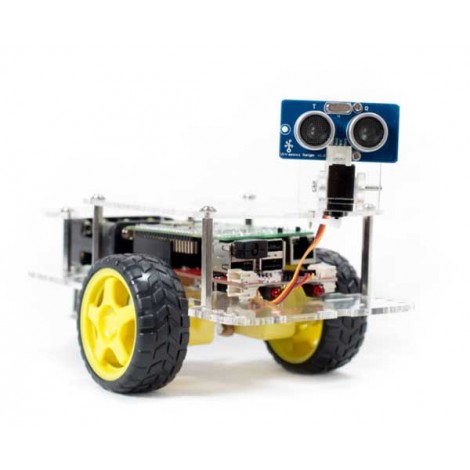
This is an implementation of Extended Kalman Filter (EKF) Simultaneous Localization and Mapping (SLAM ) using a Raspberry Pi based GoPiGo robot that is sold by Dexter Industries in kit form. The robot has two powered wheels and a third castor wheel. It is equipped with an ultrasonic range finder that is mounted on a servo mechanism that allows for the range finder to be pointed in any direction in front of the robot. An EKF SLAM implementation consists of two steps - prediction and correction. The prediction step has been implemented successfully. However, the correction step has not been fully implemented due to problems with the ultrasonic sensor as described below in the implementation details.

Problem Description

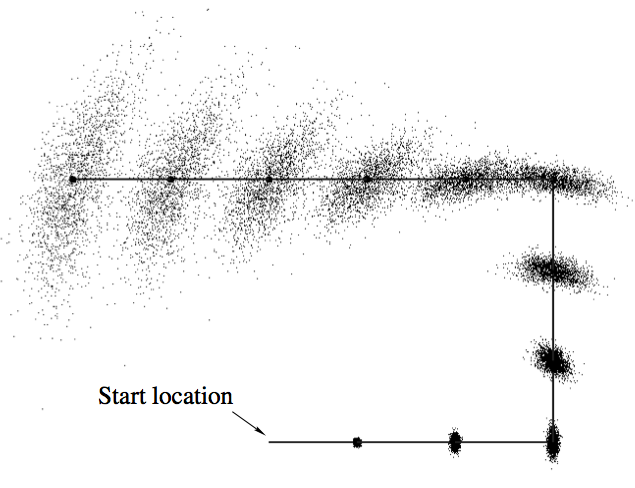
Robot motion is stochastic and not deterministic. A robot does not faithfully execute movement commands due to inaccuracies in its motion mechanism, approximations made in modeling its environment and incomplete modeling of the physics of its operating environment. Due to these reasons, the robot may not end up exactly at the location where it should have been if the movement command had been faithfully executed. The robot position may be thought of as a two dimensional probability distribution. This probability distribution will have a mean that will be equal to the expected robot location based on the movement command. The covariance will be the measure of how faithfully it executes commands. Due to this uncertainty in movement, with each motion command, the location uncertainty increases and after a while the robot gets lost.

Sampling approximation of the position belief for a non-sensing robot [3]. The solid line displays the actions, and the samples represent the robot’s belief at different points in time.

In the above diagram, before the robot starts moving, it knows exactly where it is. So it's location belief is a single point. After each movement, its location uncertainty increases. This is shown by the location probability distribution that changes from a point to a larger area with each step. In the final position of the robot, the uncertainty is the largest as it accumulates the added uncertainty with each step.

In some applications, robots need to be able to go into an unknown environment and explore it. This is a difficult problem due to the issue described above. If a map of the environment is available, the robot can use sensors to find its location in the environment. Conversely, if the robot knows where it is, it can generate an environment map. This is a sort of chicken and egg problem. Simultaneous Localization and Mapping (SLAM) solves this problem. An Extended Kalman Filter (EKF) can be used to reduce robot location uncertainty. This page describes the implementation of EKF SLAM using a robot. The EKF SLAM implementation enables the robot to keep track of its location within an environment and also create a map of the environment as it is moving.

What is a Kalman Filter

As it moves through an environment, the robot uses the knowledge of its own movement and sensing uncertainties in conjunction with an EKF to reduce its location uncertainty.

Cannonball flight smoothed out by a Kalman filter.

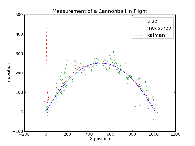
A Kalman filter is a powerful tool that can be used in environments where the data is noisy. It is able to filter out the noise and output less noisy data. A Kalman filter can be used to track objects like missiles, faces, heads, hands, navigation of ships or rockets, and many computer vision applications. Shown above is an example of the use of a Kalman filter to reduce uncertainty. A cannonball is tracked using a range-finder which returns the location with some added noise. A Kalman filter can be used to combime the expected cannonball trajectory with its location returned by a range finder to produce an good estimate of its location.

Illustration of Kalman filters (x-axis = distance moved, y-axis = probability of being at the distance) [3]: (a) initial belief, (b) a measurement (in bold) with the associated uncertainty, (c) belief after integrating the measurement into the belief using the Kalman filter algorithm, (d) belief after motion to the right (which introduces uncertainty), (e) a new measurement with associated uncertainty, and (f) the resulting belief.

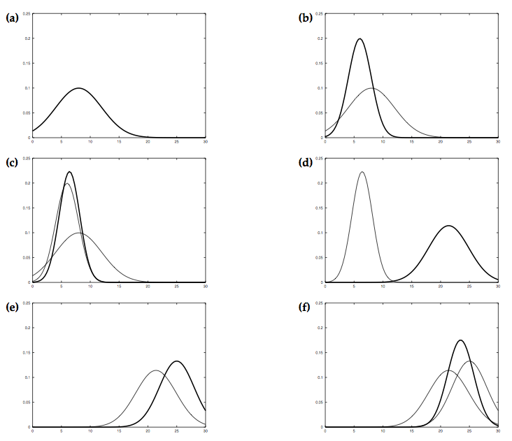
The above figure illustrates the Kalman filter for a simplistic one-dimensional localization scenario. Suppose the robot moves in the horizontal axis in each diagram with the prior over the robot localization given by the normal distribution shown in 1a. The robot queries its sensors on its location and these return a measurement that is centered at the peak of the bold Gaussian distribution in 1b. The peak corresponds to the value returned by the sensors and the its width or variance corresponds to the uncertainty in measurement. Combining the prior with the measurement yields the bold Gaussian in 1c. The belief’s mean lies between the two original means, and its uncertainty width is smaller than both contributing Gaussians. The is the result of the information gain from using the Kalman filter. Now lets assume that the robot moves towards the right. Its uncertainty grows due to the fact that the state transition is stochastic. This results in the the Gaussian shown in bold in 1d. This Gaussian is shifted by the amount the robot moved and is also wider because of the uncertainty introduced by the movement. The robot does a second sensor measurement shown in 1e, which results in the posterior shown in 1f.

Linear transformation of a Gaussian random variable [3]. The lower right plot shows the density of the original random variable, X. This random variable is passed through the function displayed in the upper right graph (the transformation of the mean is indicated by the dotted line). The density of the resulting random variable Y is plotted in the upper left graphs.

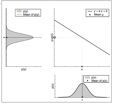
Shown above in the bottom-right part is a prior Gaussian probability distribution for a robot location and the posterior distribution on the upper-left part after it is acted on by a linear transformation. The posterior distribution is also Gaussian. In such cases a Kalman filter can be used for reducing uncertainty.

Illustration of linearization applied by the EKF [3]. Instead of passing the Gaussian through the nonlinear function, it is passed through a linear approximation of the function. The linear function is tangent to the nonlinear function at the mean of the original Gaussian. The resulting Gaussian is shown as the dashed line in the upper left graph.

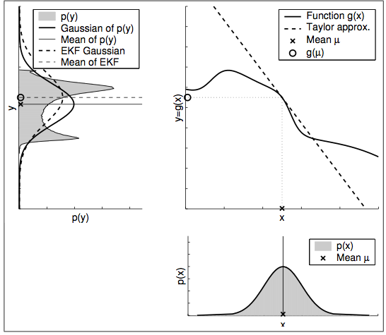
Shown above in the bottom-right part is a prior Gaussian probability distribution for a robot location and the shaded posterior distribution on the upper-left part after it is acted on by a non-linear transformation. The posterior distribution is not Gaussian. In such cases a Kalman filter cannot be used for reducing uncertainty. An extended Kalman filter can be employed by making use of a tangent to the non-linear function. The resulting Gaussian distribution is shown by the dotted line.

EKF SLAM Algorithm Details

A graphical model of the SLAM algorithm [3].

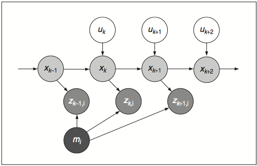
A graphical model of the SLAM algorithm is shown above. The robot pose (X coordinate, Y coordinate and robot orientation) is depicted by the circles containing the x with subscript. The circles with u and a subscript stand for the motion command at the location. The circle with m stands for a landmark and the circles with z and subscript stand for sensor measurements of the landmarks taken at the robot pose that they are attached to.

The essential SLAM problem [2]. A simultaneous estimate of both robot and landmark locations is required. The true locations are never known or measured directly. Observations are made between true robot and landmark locations.

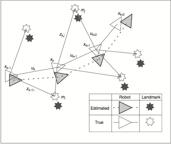
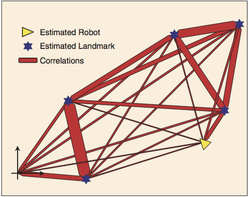
The figure above shows a robot moving through an environment, taking measurements of landmarks. As the robot does this, the estimates of the landmarks are all correlated with each other because of the common error in estimate robot location.

Spring network analogy [2]. The landmarks are connected by springs describing correlations between landmarks. As the vehicle moves back and forth through the environment, spring stiffness or correlations increase (red links become thicker). As landmarks are observed and estimated locations are corrected, these changes are propagated through the spring network. Note, the robot itself is correlated to the map.

The uncertainty reduction process can be visualized as shown above as a network of springs connecting all landmarks together or as a rubber sheet in which all landmarks are embedded. An observation in a neighborhood acts like a displacement to a spring system or rubber sheet such that its effect is great in the neighborhood and, dependent on local stiffness (correlation) properties, diminishes with distance to other landmarks. As the robot moves through this environment and takes observations of the landmarks, the springs become increasingly (and monotonically) stiffer. In the limit, a rigid map of landmarks or an accurate relative map of the environment is obtained. As the map is built, the location accuracy of the robot measured relative to the map is bounded only by the quality of the map and relative measurement sensor. In the theoretical limit, robot relative location accuracy becomes equal to the localization accuracy achievable with a given map.

(a) Example environment with three obstacles in gray. The robot is located towards the bottom of the figure and takes a measurement as indicated by the dashed line. (b) Likelihood field for this obstacle configuration. The darker the location, the less likely is the robot to perceive an obstacle there [3].

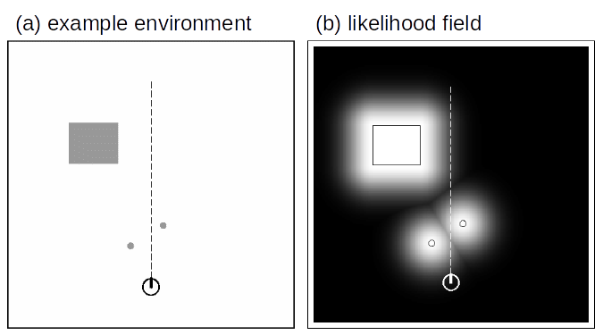
Figure (a) above shows a robot that is sensing three obstacles shown in gray in. Figure (b) shows the likelihood of the robot sensing the obstacles. The darker the location, the less likely is the robot to perceive an obstruction there. The sharp definitions of the actual obstacles are turned into blurred images that represent the uncertainty in the measurement of the obstacle coordinates and the signature. The higher the Kalman Gain, the less blurred the perceived obstacles will be.

Implementation Details

The robot manufacturer provides a Python library with movement control and rangefinder functions. The movement control functions provide for precision movement using encoders disks that are attached to the wheel axle. The robot wheels can be independently made to go forward or backward a specific number of encoder steps. The rangefinder can be pointed at any angle in front of the robot and will return the distance in centimeters to an obstacle that the sensor is pointing to. The python NumPy library has been used for matrix and array operations.

The robot has been programmed to navigate through obstacles using the rangefinder and movement commands. It first goes to the nearest obstacle and stops when it gets to within two lengths of it. Then it randomly turns 45 degrees left or right and repeats the process. Due to limitations in the ultrasonic sensor, an obstacle that is 7 cm wide is seen to be 33 cm wide. When the location and sensing uncertainty is taken into account, this will result in an obstacle with a width that will be larger than 33 cm. Due to this limitation, the distance between obstacles needed to be several times this width. This made the testing imparactical due to physical space limitations. In addition to this, the process of associating new observations to previously seen landmarks became impossible with the nearest neighbor method. The reason is that the nearest neighbor association method relies on closeness of the previously observed landmarks to their new expected location based on the robot movement. Since the sensing uncertainty is so large, it made the association with known landmarks impossible.

The final implementation of the project consists of a robot that can navigate through obstacles and can predict is current location based on its previous location plus the expected movement based on the movement command. The correction step that reduces the robot location uncertainty has not been implemented.

Project Demo

GoPiGi Obstacles Navigation from Gopal Menon on Vimeo.

References

[1] GoPiGo - Dexter Industries. Dexter Industries. N.p., n.d. Web. 06 Nov. 2015. http://www.dexterindustries.com/gopigo/.

[2] Durrant-Whyte, H., and T. Bailey, Simultaneous Localization and Map- ping: Part I, IEEE Robotics and Automation Magazine. 13.2 (2006): 99-110.

[3] Thrun, Sebastian, Wolfram Burgard, and Dieter Fox, Probabilistic Robotics, MIT press, 2005.

[4] Stachniss, Cyrill, SLAM Course - WS13/14, YouTube. YouTube, n.d. Web. 18 Sept. 2015. https://www.youtube.com/playlist?list= PLgnQpQtFTOGQrZ4O5QzbIHgl3b1JHimN_.